Convection maps
Convection maps can be plotted using the map_plot routine.
Example plot
map_plot -png \
         -coast -fcoast -mag -grd -grdontop \
         -ctr -poly -fpoly -fpolycol 554090DD \
         -extra -fit -rotate -hmb -imf -tmlbl -maxmin -pot -latmin 50 \
         -vecp -vkeyp -vkey blue+green+red+yellow.key -vsf 3 \
         -frame -dn -st 09:00 -time 20181001.north.map2
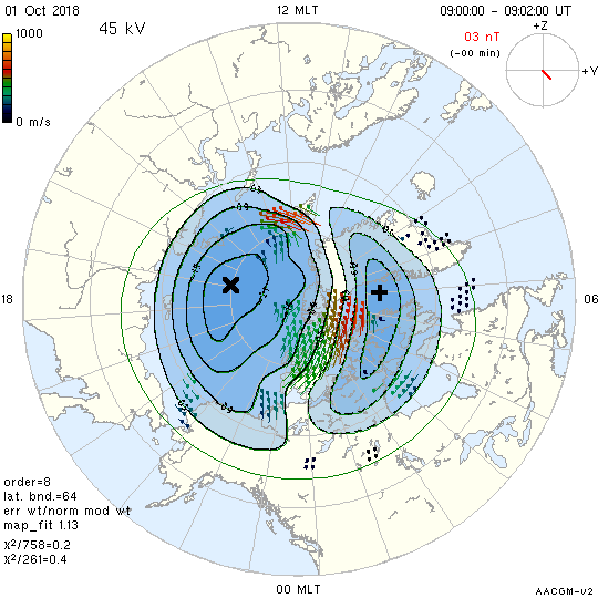
coastplot coast outlinesfcoastfill the coastlinesmaguse magnetic coordinatesgrdplot the coordinate gridgrdontopplot the grid on top of the mapped data-ctrplot the potential contours-polyplot the contour lines as polygons-fpolyfill the contour lines-fpolycol 554090DDset the color of filled contour polygons-extraplot extra diagnostic information-fitplot the fitted two-dimensional velocity vectors-rotaterotate the plot so that the local noon is at the top-hmbplot Heppner-Maynard boundary-imfplot the IMF clock-dial-tmlbllabel the time clock-dial-maxminplot the points of maximum and minimum potential-potplot the cross polar cap potential-latmin 50adjust the scale factor so that the lowest visible latitude is 50 degrees-vecpplot the example vector-vkeypplot the color key for the velocity scale-vkey blue+green+red+yellow.keyspecify which velocity color key to use-vsf 3set the vector scale factor to 3-frameadd a frame around the borders of the plot-dngenerate filenames of the form yyyymmdd.hrmn.sc.xxx-st 09:00generate plots starting at 09:00UTtimeplot the time of the plotted data
Type map_plot --help into the terminal to view all of the available input options.