The RST plotting routines should have been added to your path during installation, but you can find them in $RSTPATH/bin. You can view the available input options for each routine using, for example
time_plot --help
field_plot --help
fov_plot --help
Further examples for each function can be found in $RSTPATH/codebase/superdarn/src.bin/tk/plot/[function_name]/doc/[function_name].doc.xml
In RST you have the option to plot the data in an X-terminal, or save the plot to an image file. For example,
# Display plot in X-terminal
time_plot -x [filename].fitacf

# Produce PostScript plot as output
time_plot -ps [filename].fitacf > [filename].ps

# Produce Portable Network Graphics (PNG) image as the output
time_plot -png [filename].fitacf > [filename].png
Range time plots
Getting started
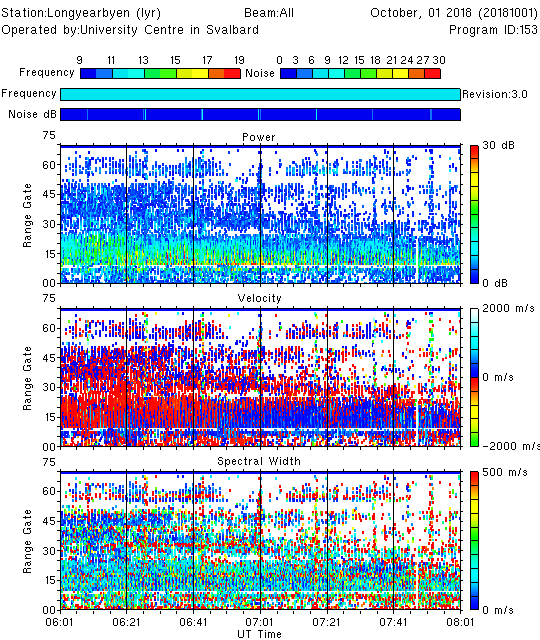
time_plot -x -a 20181001.0601.00.lyr.fitacf
An X-window showing a SuperDARN range-time plot should open.
Let's take a look at what each option means:
-xPlot the data in an X-terminal-aPlot all parameters (power, velocity, spectral width). You can plot the elevation angles by adding-e
By default, the time axis range will be determined automatically from the time span of the input file (this behavior was introduced in RST4.3). To plot a subset of the data file you have two options:
- Provide the start and end times for the time axis:
-st HH:MM -et HH:MM - Specify the start time and the interval length:
-st HH:MM -ex HH:MM
time_plot -x -a -st 06:30 -et 07:30 20181001.0601.00.lyr.fitacf
time_plot -x -a -st 06:30 -ex 01:00 20181001.0601.00.lyr.fitacf
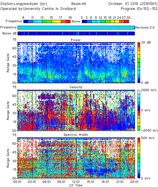
24-hour plot
Most often you will want to plot data spanning more than two hours. To achieve this, you first need to concatenate the fitacf files into a single file. With this new input file you should obtain the more familiar 24-hour range-time plot:
cat 20181001.*.lyr.fitacf > 20181001.lyr.fitacf
time_plot -x -a 20181001.lyr.fitacf
More customization options
A full list of options for customizing the range-time plots is available by typing time_plot --help, but here are a few common examples to get started. Many options can be combined together.
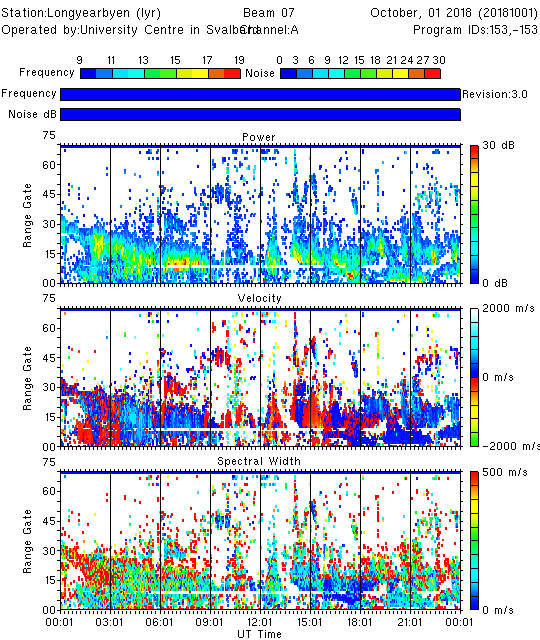
Plot only the data from channel A, beam 7
time_plot -x -a -c A -b 7 20181001.lyr.fitacf
Plot only the velocity parameter, and change the range of the color key
time_plot -x -v -vmin -500 -vmax 500 20181001.lyr.fitacf
Mark the ground scatter
time_plot -x -a -gs 20161010.lyr.fitacf
Use units of kilometers for the range axis (i.e. slant range) instead of gate number, and specify the y-axis range and major/minor tick intervals:
time_plot -x -a -km -ymajor 500 -yminor 100 -frang 0 20181001.lyr.fitacf
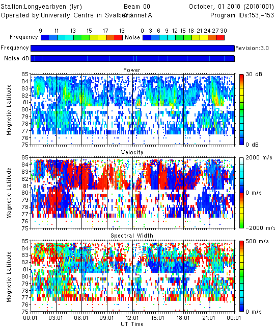
Plot magnetic latitude instead of range (or use -geo for geographic latitude)
time_plot -x -a -mag -latmin 72 -latmax 85 -b 0 -c A 20181001.lyr.fitacf
Create a PostScript output of the plot
time_plot -ps -a -xp 0 -yp 0 20181001.lyr.fitacf > timeplot.ps
The -xp 0 and -yp 0 arguments may be required for the plot to fit onto the page correctly.
Create a Portable Network Graphics (PNG) output of the plot
time_plot -png -a 20181001.lyr.fitacf > timeplot.png